Finding the Common Mode Rejection Coefficient

(an IPython notebook with the same content can be found here: https://gist.github.com/kylerbrown/a612923f1cd071c9bedd )

Assume you have two channels, A_t and B_t where t ∈ 0, 1, 2, ...T. Each channel is composed of a linear sum of a unique signal and a common noise, with the noise scaled by an unknown constant.

A_t = a_t + N_t B_t = b_t + (N_t)/(C)

If C was known, we could remove the noise from the difference of the two channels optimally, that is:

A_t − CB_t = (a_t + N_t) − C(b_t + (N_t)/(C)) = a_t − Cb_t

In paired, chonically implanted electrodes, common noise and movement artifacts can be reduced (but in practice not eliminated) using this method.

Solving for C analytically

We'd like to minimize the sum squared difference between A_n and CB_N.

SSD = ⎲⎳(A_t − CB_t)²

Taking the derivative with respect to C and setting the derivative to zero, we find

(dSSD)/(dC) = 2⎲⎳(A_t − CB_t)B_t 0 = ⎲⎳A_tB_t − C⎲⎳B²_t C = (⎲⎳A_tB_t)/(⎲⎳B²_t)

In Python, this would look something like:

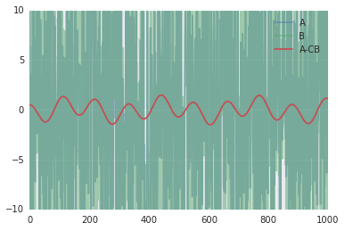
# setting up the problem
from __future__ import division
import numpy as np
T = 1000
t = np.arange(T)
common_noise = 10*np.random.randn(T)
true_C = .5
signal_1 = np.cos(2*np.pi*t/110)
signal_2 = np.cos(2*np.pi*t/300)
A = signal_1 + common_noise
B = signal_2 + common_noise / true_C

# solving for C
C = np.dot(A, B) / np.dot(B, B)
print("True C: {}, computed C {}".format(true_C, C))

True C: 0.5, computed C 0.499955696052

import matplotlib.pyplot as plt
import seaborn as sns
%matplotlib inline
plt.plot(A, alpha=.5, label="A")
plt.plot(B, alpha=.5, label="B")
plt.plot(A-C*B, label="A-CB")
plt.legend()
plt.ylim(-10,10);

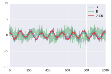
Interestingly, this method works less well with a lower noise channels, for example:

common_noise = 0.5*np.random.randn(T)
A = signal_1 + common_noise
B = signal_2 + common_noise / true_C
C = np.dot(A, B) / np.dot(B, B)
print("True C: {}, computed C {}".format(true_C, C))

True C: 0.5, computed C 0.350776916893

plt.plot(A, alpha=.5, label="A")
plt.plot(B, alpha=.5, label="B")
plt.plot(A-C*B, label="A-CB")
plt.legend()
plt.ylim(-10,10);

Solving for C using optimization

We can use optimization packages, such as scipy's optimize module to check our analytical solution.

from scipy.optimize import minimize
def SSD (c, a, b):
    """returns the sum squared of a - c*b"""
    return np.sum( (a-c*b)**2 )

res = minimize(SSD, 1, args=(A, B))
C = res.x[0]
print("True C: {}, computed C: {}".format(true_C, C))

True C: 0.5, computed C: 0.350776907985

Which is the same solution found analytically.

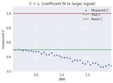
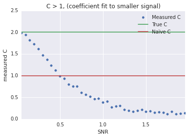
Quality of common mode rejection over signal-to-noise ratios

def find_c(snr, T, true_C):
    signal_1 = np.random.randn(T)
    signal_2 = np.random.randn(T)
    common_noise = 1/snr*np.random.randn(T)
    A = signal_1 + common_noise
    B = signal_2 + common_noise / true_C
    return np.dot(A, B) / np.dot(B, B)

true_C = 0.5
snr = np.arange(0.05, 2, 0.05)
C = [find_c(x, 1000, true_C) for x in snr]
plt.scatter(snr, C, label="Measured C", color=sns.color_palette()[0])
plt.xlabel("SNR")
plt.ylabel("measured C")
plt.hlines(true_C, snr[0], snr[-1], label="True C", color=sns.color_palette()[1])
plt.hlines(1, snr[0], snr[-1], label=u"Naïve C",
           color=sns.color_palette()[2])
plt.legend()
plt.xlim(snr[0], snr[-1])
plt.title("C < 1, (coefficient fit to larger signal)");

true_C = 2
snr = np.arange(0.05, 2, 0.05)
C = [find_c(x, 1000, true_C) for x in snr]
plt.scatter(snr, C, label="Measured C", color=sns.color_palette()[0])
plt.xlabel("SNR")
plt.ylabel("measured C")
plt.hlines(true_C, snr[0], snr[-1], label="True C", color=sns.color_palette()[1])
plt.hlines(1, snr[0], snr[-1], label=u"Naïve C",
           color=sns.color_palette()[2])
plt.legend()
plt.xlim(snr[0], snr[-1])
plt.title("C > 1, (coefficient fit to smaller signal)");

Conclusion

Optimizing C works best when the SNR is low, so a segment of recording without much signal is ideal. When fitting C, choose the noiser of the two channels.